Introduction
Database Systems VS File Systems
Problems with file systems:
- Longer development times.
- Longer time to get answers about data.
- Complex system administration.
- Security issues which are harder to manage.
- Extensive programming.
- Structural dependence.
Problems with Database systems:
- Increased costs.
- Management complexity.
- Maintaining currency.
- Vendor dependence.
- Frequent upgrade/replacement cycles.
Basic Terminology
- Data: Raw facts. Data has little meaning unless they have been organized into some logical arrangement.
- Field: A character or group of characters that has a specific meaning. A field is used to define and store data.
- Record: A logically connected set of one or more fields that describes a person, place, or thing.
- File: A collection or related records.
Structural Dependence
- Structural dependence: Access to file is dependent on its structure. All file system programs need to be modified to conform to a new file structure.
- Structural independence: File structure can be changed without affecting the application's ability to access the data.
Data Dependence
- Data dependence: Data access changes when data storage characteristics change.
- Data independence: Data storage characteristics is changed without affecting the program's ability to access the data.
Data Redundancy
Unnecessarily storing same data at different places. Islands of information is when data is scattered in locations. This increases the probability of having different version of the same data.
Problems
- Poor Data security.
- Data inconsistency.
- Increased likelihood of data-entry errors when complex entries are made in different files.
- Data anomaly: Develops when not all the required changes in the redundant data are made successfully.
Data Anomaly
- Update Anomalies
- Insertion Anomalies
- Deletion Anomalies
Types of Databases
By Users
- Single-user database: Supports one user at a time.
- Desktop database: Runs on a personal computer.
- Multi-user database: Supports multiple users at the same time.
- Workgroup database: Supports a small number of users or a specific department.
- Enterprise database: Supports many users across many departments.
By Location
- Centralized database: Data is located at a single site.
- Distributed database: Data is distributed across different sites.
- Cloud database: Created and maintained using cloud data services that provide defined performance measures for the database.
By Purpose
- General-purpose database: Contains a wide variety of data used in multiple disciplines.
- Discipline-specific databases: Contains data focused on specific subject areas.
By Time Sensitivity and Use
- Operational database: Designed to support a company's day-to-day operations. (Also called Online transaction processing database (OLTP)).
- Analytical database: Stores historical data and business metrics used exclusively for tactical or strategic decision-making.
- Data warehouse: Stores data in a format optimized for decision support.
- Online analytical processing (OLAP): Tools for retrieving processing, and modeling data from the data warehouse.
- Business intelligence: Captures and process business data to generate information that support decision making.
By Structure
- Unstructured data: It exists in their original state.
- Structured data: It results from formatting.
- Semi-structured data: Processed to some extent.
- Extensible Markup Languages (XML): Represents data elements in textual format.
ACID VS BASE Transactions
ACID
ACID: Atomicity, Consistency, Isolation, Durability.
- Atomicity: Each transaction is all or nothing (Transaction can consist of multiple commands)
- Consistency: Any transaction brings the database from one valid state to another.
- Isolation: Concurrent execution of statements would be if those statements were executed sequentially.
- Durability: Once a transaction has been committed, it will remain so, even in the event of power loss, crashes or breakdowns.
The ACID model ensures data is safe and consistently stored. Normally employed by Relational databases.
BASE
BASE: Basic, Availability, Soft state, Eventual consistency
- Basic Availability: System guarantees availability as regards the CAP (Consistency, Availability, Partition tolerance)
- Soft state: System state could change over time, even without input, due to Eventual consistency.
- Eventual consistency: System will eventually become consistent when it stops receiving input.
The BASE model prioritize availability over consistency. Normally employed by NoSQL databases.
Data Modeling
Data modeling is a process used to define and analyze data requirements needed to support the business process within the scope of corresponding information systems in organizations.
Iterative and progressive process of creating a specific data model for a determined problem domain.
Data models are simple representations of complex real world data structures.
Types
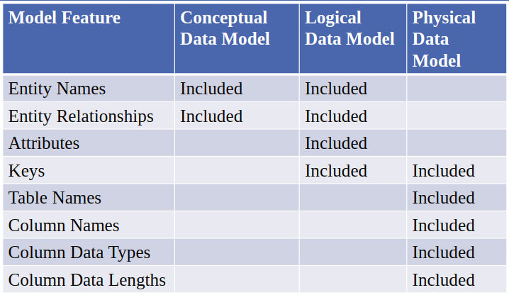
Conceptual Data Model
- Identifies the highest-level relationship between entities.
- Facilitates communication, and integration between systems, processes, and organizations.
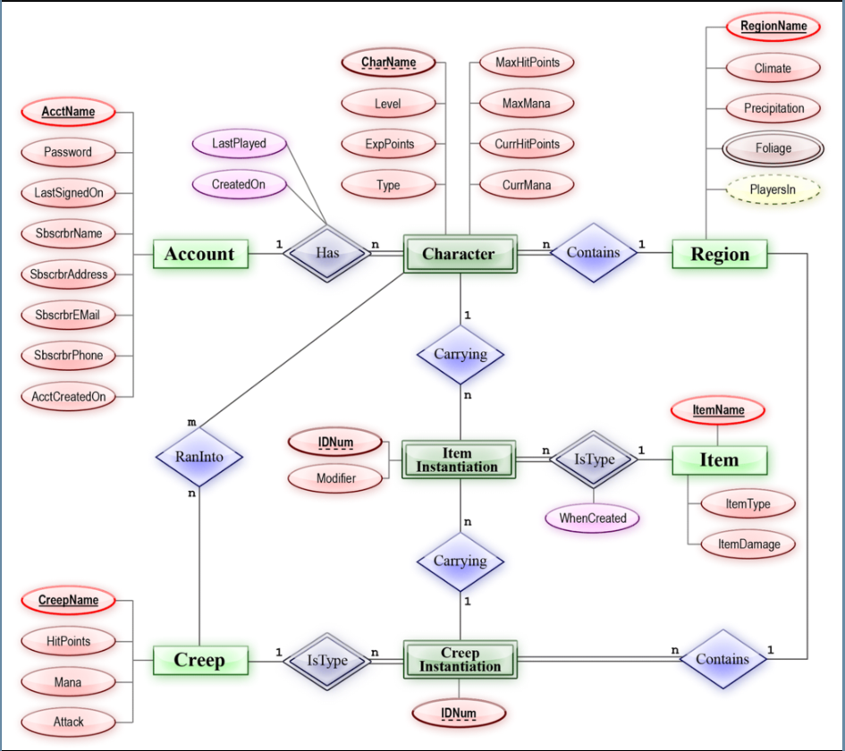
- Often expressed using an entity-relationship model (ERM).
Logical Data Model
- Expands on the CDM (conceptual data model) with more details.
- Describes the data in as much detail as possible, without regards to its physical implementation.
- Contains attributes in addition to entities and relationship.
- Normalization done at this level.
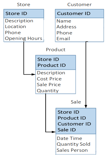
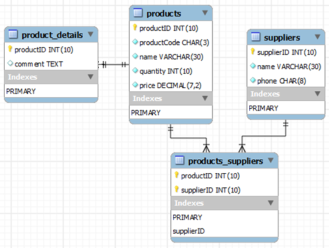
Physical Data Model
- Models how actual database will be build.
- Shows the complete table structure, keys, and relationships between tables.
- Dependent on the database management systems used.
Basic Building Blocks
- Entity: Unique and distinct object used to collect and store data.
- Attribute: Characteristic of an entity.
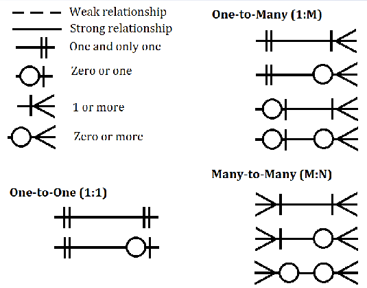
- Relationship: Describes an association among entities.
- One-to-many (1:M)
- Many-to-many (M:N or M:M)
- One-to-one (1:1)
- Constraint: set of rules to ensure data integrity.
Types of Relationships
Terminology
- Key attribute: Attribute that is a part of a key.
- Entity integrity: Condition in which each row in the table has its own unique identity.
- Referential integrity: Every reference to an entity instance by another entity instance is valid.
Integrity Rules
- Entity Integrity
- All PK entries are unique, and no part of a PK may be null.
- Each row will have a unique identity, and foreign key (FK) values can properly reference PK values.
- Referential Integrity
- FK may or may not be part of its table's PK.
- FK may be null, if it's not a part of the PK.
- Every non-null FK value must reference an existing PK value in the table to which it's related.
SQL
SQL is a non-procedural language (you command what is to be done, not how it is to be done.) SQL commands are broadly into DDL and DML commands. DDL commands are used to configure the structure of the database and tables. DML commands are used to modify data within those tables and structures.
DDL (Data Definition Language)
Data Definition Language is used to work with structure in SQL. DDL includes commands to create database objects such as tables, indexes, and views; define constrains for data objects; define access rights to the database objects.
Create Database/Schema
CREATE SCHEMA schema_name AUTHORIZATION creator;
The keyword DATABASE can be used instead of SCHEMA.
Optionally, can use [IF NOT EXISTS] to prevent error message if database already exists.
CREATE DATABASE IF NOT EXISTS my_first_database;
Create Table Structures
CREATE TABLE tablename (
    column1     datatype    [constraint],
    column2     datatype    [constraint],
    PRIMARY KEY (column1 [, column2]),
    FOREIGN KEY (column1 [, column2])
        REFERENCES tablename2 (column1[, column2]),
    CONSTRAINT  constraint1
);
Example:
CREATE TABLE `country` (
    `Code`        char(3)       NOT NULL    DEFAULT "",
    `Name`        varchar(52)   NOT NULL    DEFAULT "",
    `Continent`   varchar(52)   NOT NULL    DEFAULT "",
    `Population`  int                       DEFAULT "Africa",
    `LifeExp`     float(3,1)                DEFAULT NULL,
    `Capital`     varchar(52)               DEFAULT NULL,
    PRIMARY KEY (`Code`)
);
SQL Constraints
NOT NULL: Ensures that column does not accept nulls.UNIQUE: Ensures that all values in column are unique.DEFAULT: Assigns value to attribute when a new row is added to table.CHECK: Validates data when attribute value is entered.
Examples:
CONSTRAINT CUSTOMER_NAME_UNIQ UNIQUE(CUS_LNAME, CUS_FNAME);

CONSTRAINT INVOICE_CHECK CHECK(INV_DATE > TO_DATE('01-JAN-2016', 'DD-MON-YYYY'));
SQL Data Types
NUMBER(L, D) or NUMERIC(L, D): L is the number of character and D is the number of digits after the decimal place.INTEGER or INT: Used to store integers.SMALLINT: Like INT but limited to integer values up to six digits.DECIMAL(L, D): Like NUMBER specification, but the storage length is a minimum specification. Greater lengths are acceptable.CHAR(L): Fixed-length character data for up to 255 characters.VARCHAR(L) or VARCHAR2(L): Variable-length character data.DATE: Stores dates in the Julian date format.DATETIME: Used for values that contain both date and time parts.TIMESTAMP: Used to record the date and time of an event.
Alter Table Structure
We can use the ALTER TABLE command to make changes to the table structure:
ADD: Adds a column.MODIFY: Changes column characteristics.DROP: Delete a column.
Also used to:
- Add table constraints.
- Remove table constraints.
Adding and Dropping Columns
ALTER TABLE tablename ADD (column datatype);

ALTER TABLE tablename MODIFY column datatype;

ALTER TABLE tablename DROP COLUMN column;

ALTER TABLE tablename RENAME column TO column2;

ALTER TABLE tablename CHANGE column to column2 datatype;
Renaming and Dropping Table from the Database
RENAME TABLE tablename TO newtablename;

DROP TABLE tablename;
Can drop a table only if it is not the one side of any relationship. RDBMS generates a foreign key integrity violation error message if you try to drop a referenced table.
| Command or Option |
Description |
| CREATE SCHEMA AUTHORIZATION |
Creates a database schema |
| CREATE TABLE |
Creates a new table in the user's database schema |
| NOT NULL |
Ensures that a column will not have null values |
| UNIQUE |
Ensures that a column will not have duplicate values |
| PRIMARY KEY |
Defines a primary key for a table |
| FOREIGN KEY |
Defines a foreign key for a table |
| DEFAULT |
Defines a default value for a column (when no value is given) |
| CHECK |
Validates data in an attribute |
| CREATE INDEX |
Creates an index for a table |
| CREATE VIEW |
Creates a dynamic subset of rows and columns from one or more tables |
| ALTER TABLE |
Modifies a table's definition (adds, modifies, or deletes attributes or constraints) |
| CREATE TABLE AS |
Creates a new table based on a query in the user’s database schema |
| DROP TABLE |
Permanently deletes a table (and its data) |
| DROP INDEX |
Permanently deletes an index |
| DROP VIEW |
Permanently deletes a view |
DML (Data Manipulation Language)
DML is used to query and manage the data inside the database. They include commands to insert, update, and delete data within the database table. It also includes commands to query the database and return useful information.
Adding Data to a Table
INSERT INTO tablename VALUES (value1, value2, ..., valueN);

INSERT INTO tablename (column1, ..., columnN) VALUES (value1, ..., valueN);
The second statement can be used to add a subset of all the columns.
Updating Table Data
UPDATE tablename SET assignment_list [WHERE where condition];
Example:
UPDATE country SET LifeExp = 100;
UPDATE country SET LifeExp = 79.4 WHERE Code="CAN";
Deleting Table Rows
DELETE FROM tablename [WHERE condition];
Select Statements
Here is the most basic version of the select statement:
SELECT columnlist FROM tablename;
Example:
SELECT * FROM country;
SELECT Code, Name FROM country;
WHERE Conditional
We can use the WHERE conditional along with comparison operators and logical operators to filter our select statement.
WHERE column1 = column2 AND colum3 >= value1;

-- Example
WHERE first = last AND code >= 200;
Multiple Tables
There are many ways in SQL to get data from many tables and the act of connecting 2 tables is called a "JOIN".
Cross Join
A cross-join returns the Cartesian product of the two tables.
-- Old style
SELECT * FROM T1, T2;

-- New style
SELECT * FROM T1 CROSS JOIN T2;
Inner Join
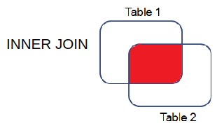
Natural Join
Returns only the rows with matching values in the matching columns; the matching columns must have the same names and similar data types.
SELECT * FROM T1 NATURAL JOIN T2;
Natural joins aren't recommended because:
- DBMS 'guesses' columns to join based on name and type.
- Harder to maintain and document.
- JOINs cannot be done if column names are different.
- Always an Equi-Join i.e. based on equality.
Join Using
Returns only the rows with the matching values in the columns indicated in the USING clause.
SELECT * FROM T1 FROM T2 USING (C1 [, C2]);
Join On
Returns only the rows that meet the join condition indicated in the ON clause.
SELECT * FROM T1 JOIN T2 ON T1.C1 = T2.C2;
Outer Join
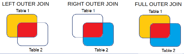
Left Join
Return rows with matching values and includes all rows from the left table (T1) with unmatched values. The best way to think of this is: we have a table T1, and we're trying to append the data from T2 onto T1.
SELECT * FROM T1 LEFT OUTER JOIN T2 ON T1.c1 = T2.c1;

SELECT * FROM T1 LEFT JOIN T2 ON T1.c1 = T2.c1;
Right Join
Return rows with matching values and includes all rows from the right table (T2) with unmatched values. The best way to think of this is: we have a table T2, and we're trying to append the data from T1 onto T2.
SELECT * FROM T1 RIGHT OUTER JOIN T2 ON T1.c1 = T2.c1;

SELECT * FROM T1 RIGHT JOIN T2 ON T1.c1 = T2.c1;
Full Join
Return rows with matching values and includes all rows from both tables (T1 and T2) with unmatched values.
SELECT * FROM T1 FULL OUTER JOIN T2 ON T1.c1 = T2.c1;
Transactions
START TRANSACTION;

COMMIT [work];
These 2 commands are used when committing changes to the database.
Restoring Table Contents
The ROLLBACK command can be used to restore the previous state of the database.
COMMIT and ROLLBACK only work with the data manipulation commands that add, modify or delete data rows.
Operators and Functions
Comparison Operators
| Symbol |
Meaning |
| = |
Equal To |
| < |
Less than |
| > |
greater than |
| <= |
Less than or equal |
| >= |
Greater than or equal |
| <> or != |
Not Equal |
Logical Operators
OR: logical or operation on 2 comparisons.AND: logical and operation on 2 comparisons.NOT: negate the result of a comparison.
Arithmetic Operators
+: Add.-: Subtract.*: Multiply./: Divide.^: Power of.
Numeric Functions
Find all numeric functions at this link: Numeric Functions.
String Functions
Find all string functions at this link: String Functions
Date Time Functions
Find all date time functions at this link: Date Time
Functions
Subqueries
Subqueries are used when it is necessary to process data based on other processed data.
Example: "Provide a list of vendors who do not provide any products."
select V_CODE, V_NAME from VENDOR where V_CODE not in
    (select V_CODE from PRODUCTS);
A subquery is a query (select statement) inside another query. The first query is often known as the outer query and the subquery is known as the inner query.
Inner queries are executed first. And the entire SQL statement is referred to as a nested query.
Returns a list of values
When a subquery returns a list of values (usually one column) we can use keywords like: IN, ANY, ALL to ask questions about this list.
Examples:
SELECT P_CODE, P_PRICE FROM PRODUCT
    WHERE P_PRICE IN
    (SELECT P_PRICE FROM PRODUCT WHERE V_CODE=23119);

SELECT P_CODE, P_PRICE FROM PRODUCT
    WHERE P_PRICE > ANY
    (SELECT P_PRICE FROM PRODUCT WHERE V_CODE=23119);

SELECT P_CODE, P_PRICE FROM PRODUCT
    WHERE P_PRICE > ALL
    (SELECT P_PRICE FROM PRODUCT WHERE V_CODE=23119);
Correlated subqueries executes once for each row in the outer query. This makes this extremely slow.
Example:
SELECT INV_NUMBER, P_CODE, LINE_UNITS FROM LINE L1
    WHERE L1.LINE_UNITS > (
        SELECT AVG(LINE_UNITS)
        FROM LINE L2
        WHERE L1.P_CODE=L2.P_CODE
    );
In the above example, we can see that L1.P_CODE is used from the outer query inside the inner query. This makes this query a correlated subquery.
Control Flow and Conditional Expressions
CASE Expressions
A CASE expression is used when we need to return different results based on a condition or the result of a value or expression.
There are 2 formats of the CASE statement:
CASE value
    WHEN compare_value THEN result
    [WHEN compare_value THEN result] ...
    [ELSE result]
END
CASE
    WHEN [condition] THEN result
    [WHEN [condition] THEN result ...]
    [ELSE result]
END
If function
Evaluates an expression to TRUE or FALSE and retuns different expressions based on the result of this evaluation.
IF (expr1, expr2, expr3)

-- If expr1 is true (not 0 or null),
-- return expr2, otherwise return expr3
Example of useful case:
SELECT
    COUNT(IF(P_DISCOUNT>0, 1, NULL)) as 'Discounted',
    COUNT(IF(P_DISCOUNT=0, 1, NULL)) as 'Not discounted'
FROM PRODUCT;
Views
A virtual table is the output of a relational operator such as a SELECT is another relation (or table).
A View is a virtual table based on a SELECT query. The tables on which the query is based are called base tables.
We can create views in mysql using the CREATE VIEW command.
CREATE VIEW viewname AS SELECT query
Create view is classified as a DDL command since it stores the sub-query specification in the data dictionary.
Example: "Create a view to generate the product listing with the quantity on hand of products with price over 50".
CREATE VIEW price_gt_50 AS
    SELECT p_descript, p_qoh, p_price
    FROM product
    WHERE p_price > 50;


-- View data using the created view
select * from price_gt_50;
Since views are stored SELECT statements posing as a table, the actual data is only stored in the original tables.
Updatable views can be updated, not all views are updatable. An updatable view is a view that does not contain any of the following:
- Aggregate function or
GROUP BY expression.
SET operators like UNION, INTERSECT or MINUS.- Views without all
NOT NULL columns from the base tables.
We can see which views are updatable in mysql using the following command:
SELECT TABLE_NAME, IS_UPDATABLE
    FROM INFORMATION_SCHEMA.VIEWS
    WHERE TABLE_SCHEMA = 'schema name';
Indexes
In computer science, a term index is a data structure to facilitate fast lookup of terms and clauses in a logic program, deductive database.
These are used to quickly find rows with specific column values.
- Index key: Index's reference point that leads to data location identified by the key.
- Unique index: Index key can have only one pointer value associated with it.
Each index is associated with only one table. One table can have several indexes. Index is automatically created on the primary key column.
Indexes result in faster searches but slower updates. This is because every time a value in the table (associated with an index) is updated then all the corresponding indexes must be recomputed as well.
We can use the CREATE INDEX command to create an index. The UNIQUE qualifies prevents a value that has been used before. Composite indexes prevent data duplication.
To delete an index, use the DROP INDEX command.
Syntax:
CREATE [UNIQUE] INDEX indexname
    ON tablename (col1 [, col2]);
Examples:
-- Creates index on column P_CODE
CREATE UNIQUE INDEX P_CODEX
ON PRODUCT (P_CODE);

-- Creates index in desc. order
CREATE INDEX PROD_PRICEX
ON PRODUCT (P_PRICE DESC);
Procedural SQL
-
Standard SQL lacks procedural functionality, it does not support conditional (IF, ELSE) statements or loops (WHILE, FOR).
-
SQL-99 standard defines the use of persistent stored modules (PSM). A block of code containing standard SQL statements and procedural extensions. The code is executed at the DBMS sever.
-
Support for PSMs is left up to the vendors. PMSs existed long before they were standardized. Different vendors implement a similar procedure is different ways.
Stored Procedures
A stored procedure is a collection of procedural and SQL statements. These statements are stored in the database just like tables, views and triggers.
These procedures can be used to encapsulate and represent business transactions.
Advantages of Stored procedures
-
Reduced network traffic (no transmission of individual SQL statements over the network).
-
Increased performance (All transactions are executed locally on the server).
-
Encapsulation and security (Column names of the table are hidden, and execution privileges to users can be granted.)
-
Change in table structure will not affect code.
Example of a stored procedure without input and output:
DELIMITER //

CREATE PROCEDURE allMovies()
BEGIN
    select title, description from film;
END //

DELIMITER ;
Note, in the above example we reset the delimiter so that we can use ; for statements within the stored procedure. Once we're done with our stored procedure, we reset our delimiter to the semicolon.
We can view all stored procedures by running:
select routine_name, routine_type,definer,created,security_type,SQL_Data_Access from information_schema.routines where routine_type='PROCEDURE' and routine_schema='name_of_schema';
Delete a procedure:
DROP PROCEDURE <procedure-name>;
Parameterized Stored Procedure
When we create a stored procedure, the parameters must be specified within the parenthesis. The syntax is as follows:
(IN | OUT | INOUT) (Parameter Name [datatype(length)])
Example of IN params
DELIMITER //
CREATE PROCEDURE moviesByRating(IN rating varchar(50))
BEGIN
    select title, description from film where rating=rating;
END //
DELIMITER ;
Example of OUT params
DELIMITER //
CREATE PROCEDURE countPG13(OUT Total_Movies int)
BEGIN
    select count(title) INTO Total_Movies from film where rating='PG-13';
END //
DELIMITER ;
Example of using such a procedure:
CALL countPG13(@totalPG13);
select @totalPG13 as Movies;
Keys
- Super key: Any combination of columns that uniquely identify the entire row
- Candidate key: all minimal super keys
- Primary key
- Alternate keys